李沐动手学深度学习系列-From 0 To Softmax简介回归实现

In [21]:


import numpy as np
import torch
from torch.utils import data
import torchvision
from torchvision import transforms

In [25]:


x=torch.arange(4.0)
x

Out[25]:


tensor([0., 1., 2., 3.])

In [35]:


# 需要存梯度
x.requires_grad_(True)
# 点积
y=2*torch.dot(x,x)
# 反向传播
y.backward()
y,x.grad

Out[35]:


(tensor(28., grad_fn=<MulBackward0>), tensor([ 0.,  4.,  8., 12.]))

In [34]:


# 注意：多次运行会积累梯度x.grad的值会越来越大，最后导致梯度爆炸，导致模型无法收敛。
# 清空梯度
x.grad.zero_()

Out[34]:


tensor([0., 0., 0., 0.])

In [37]:


x.grad==4.0 * x

Out[37]:


tensor([True, True, True, True])

In [40]:


x.grad.zero_()
y=x*x
y.sum().backward()
x.grad==2*x

Out[40]:


tensor([True, True, True, True])

In [ ]:


# 非标量变量的反向传播
# 当y不是标量时，向量y关于向量x的导数的最自然解释是一个矩阵。 对于高阶和高维的y和x，求导的结果可以是一个高阶张量。

# 然而，虽然这些更奇特的对象确实出现在高级机器学习中（包括深度学习中）， 但当调用向量的反向计算时，我们通常会试图计算一批训练样本中每个组成部分的损失函数的导数。 这里，我们的目的不是计算微分矩阵，而是单独计算批量中每个样本的偏导数之和。

# 对非标量调用backward需要传入一个gradient参数，该参数指定微分函数关于self的梯度。
# 本例只想求偏导数的和，所以传递一个1的梯度是合适的
x.grad.zero_()
y = x * x
# 等价于y.backward(torch.ones(len(x)))
y.sum().backward()
x.grad

In [ ]:


# 一些相关概念
# 梯度下降 就是梯度下降的意思(gradient descent) ，不断求导进行求解
# 超参数就是学习率(learning rate) (hyper-parameter)
# 学习率不能太大，否则会导致梯度爆炸，导致模型无法收敛。学习率不能太小，否则会导致模型收敛过慢。
# 随机采样样本的平均损失，实现小批量梯度下降
# 批次大小(batch size) 就是一次迭代所用的样本数目
# 随机梯度下降(stochastic gradient descent) 就是随机每次只用一个样本进行梯度下降

In [44]:


# 线性回归的简洁实现
from d2l import torch as d2l
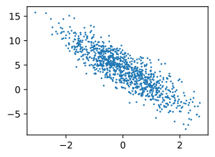
true_w = torch.tensor([2, -3.4])
true_b = 4.2
# 根据带有噪声的线性模型生成数据集
features,labels=d2l.synthetic_data(true_w,true_b,1000)
features[0],labels[0]
d2l.set_figsize()
d2l.plt.scatter(features[:,1].detach().numpy(),labels.detach().numpy(),1)

Out[44]:


<matplotlib.collections.PathCollection at 0x18ea1288290>

[

](https://img2024.cnblogs.com/blog/3517150/202505/3517150-20250519230111209-921655458.svg)

In [ ]:


# 读取数据
def load_array(data_arrays, batch_size, is_train=True):  #@save
    """构造一个PyTorch数据迭代器"""
    dataset = data.TensorDataset(*data_arrays)
    return data.DataLoader(dataset, batch_size, shuffle=is_train)
batch_size = 10
data_iter = load_array((features, labels), batch_size)
next(iter(data_iter))

Out[ ]:


[tensor([[ 0.4169, -0.4563],
         [-0.3045,  1.5433],
         [ 1.8890, -0.1051],
         [-1.3187,  1.4942],
         [ 0.0831, -0.6467],
         [ 0.4098,  1.1697],
         [ 0.4598, -0.4584],
         [ 0.1202, -0.4323],
         [ 0.6556, -0.0918],
         [ 0.0445, -1.0100]]),
 tensor([[ 6.5691],
         [-1.6594],
         [ 8.3287],
         [-3.5170],
         [ 6.5659],
         [ 1.0474],
         [ 6.6821],
         [ 5.9232],
         [ 5.8114],
         [ 7.7147]])]

In [51]:


# 开始一个最简单的神经网络模型，线性回归模型
# nn 是torch的神经网络模块
from torch import nn
# Sequential 是nn的容器模块，可以将多个网络层组合成一个网络
net=nn.Sequential(nn.Linear(2, 1))  # 线性回归模型
net[0].weight.data.normal_(0, 0.01)  # 初始化权重，均值为0，标准差为0.01
net[0].bias.data.fill_(0)  # 初始化偏差为0
loss=nn.MSELoss()  # 均方误差损失函数
optimizer=torch.optim.SGD(net.parameters(), lr=0.03)  # 随机梯度下降优化器,learning rate为0.03
for epoch in range(100):
    for X, y in data_iter:
        # 前向传播
        y_hat = net(X)
        l = loss(y_hat, y.view(-1,1))  # 损失函数
        # 梯度清零
        optimizer.zero_grad()
        # 反向传播
        l.backward()
        # 更新参数
        optimizer.step()
    l = loss(net(features), labels.view(-1,1))
    print(f'epoch {epoch + 1}, loss {l:f}')
# 预测


epoch 1, loss 0.000368
epoch 2, loss 0.000097
epoch 3, loss 0.000099
epoch 4, loss 0.000097
epoch 5, loss 0.000098
epoch 6, loss 0.000097
epoch 7, loss 0.000099
epoch 8, loss 0.000098
epoch 9, loss 0.000097
epoch 10, loss 0.000098
epoch 11, loss 0.000097
epoch 12, loss 0.000097
epoch 13, loss 0.000098
epoch 14, loss 0.000097
epoch 15, loss 0.000097
epoch 16, loss 0.000097
epoch 17, loss 0.000097
epoch 18, loss 0.000097
epoch 19, loss 0.000098
epoch 20, loss 0.000097
epoch 21, loss 0.000097
epoch 22, loss 0.000097
epoch 23, loss 0.000097
epoch 24, loss 0.000097
epoch 25, loss 0.000097
epoch 26, loss 0.000097
epoch 27, loss 0.000097
epoch 28, loss 0.000097
epoch 29, loss 0.000097
epoch 30, loss 0.000098
epoch 31, loss 0.000097
epoch 32, loss 0.000097
epoch 33, loss 0.000098
epoch 34, loss 0.000098
epoch 35, loss 0.000098
epoch 36, loss 0.000097
epoch 37, loss 0.000097
epoch 38, loss 0.000097
epoch 39, loss 0.000097
epoch 40, loss 0.000097
epoch 41, loss 0.000099
epoch 42, loss 0.000098
epoch 43, loss 0.000098
epoch 44, loss 0.000097
epoch 45, loss 0.000097
epoch 46, loss 0.000097
epoch 47, loss 0.000097
epoch 48, loss 0.000097
epoch 49, loss 0.000098
epoch 50, loss 0.000097
epoch 51, loss 0.000097
epoch 52, loss 0.000097
epoch 53, loss 0.000097
epoch 54, loss 0.000097
epoch 55, loss 0.000098
epoch 56, loss 0.000097
epoch 57, loss 0.000098
epoch 58, loss 0.000097
epoch 59, loss 0.000097
epoch 60, loss 0.000097
epoch 61, loss 0.000097
epoch 62, loss 0.000098
epoch 63, loss 0.000097
epoch 64, loss 0.000097
epoch 65, loss 0.000097
epoch 66, loss 0.000097
epoch 67, loss 0.000098
epoch 68, loss 0.000097
epoch 69, loss 0.000097
epoch 70, loss 0.000098
epoch 71, loss 0.000097
epoch 72, loss 0.000098
epoch 73, loss 0.000097
epoch 74, loss 0.000097
epoch 75, loss 0.000097
epoch 76, loss 0.000098
epoch 77, loss 0.000097
epoch 78, loss 0.000097
epoch 79, loss 0.000097
epoch 80, loss 0.000097
epoch 81, loss 0.000098
epoch 82, loss 0.000098
epoch 83, loss 0.000097
epoch 84, loss 0.000098
epoch 85, loss 0.000098
epoch 86, loss 0.000098
epoch 87, loss 0.000097
epoch 88, loss 0.000097
epoch 89, loss 0.000098
epoch 90, loss 0.000097
epoch 91, loss 0.000097
epoch 92, loss 0.000097
epoch 93, loss 0.000098
epoch 94, loss 0.000097
epoch 95, loss 0.000097
epoch 96, loss 0.000097
epoch 97, loss 0.000097
epoch 98, loss 0.000097
epoch 99, loss 0.000098
epoch 100, loss 0.000097

In [ ]:


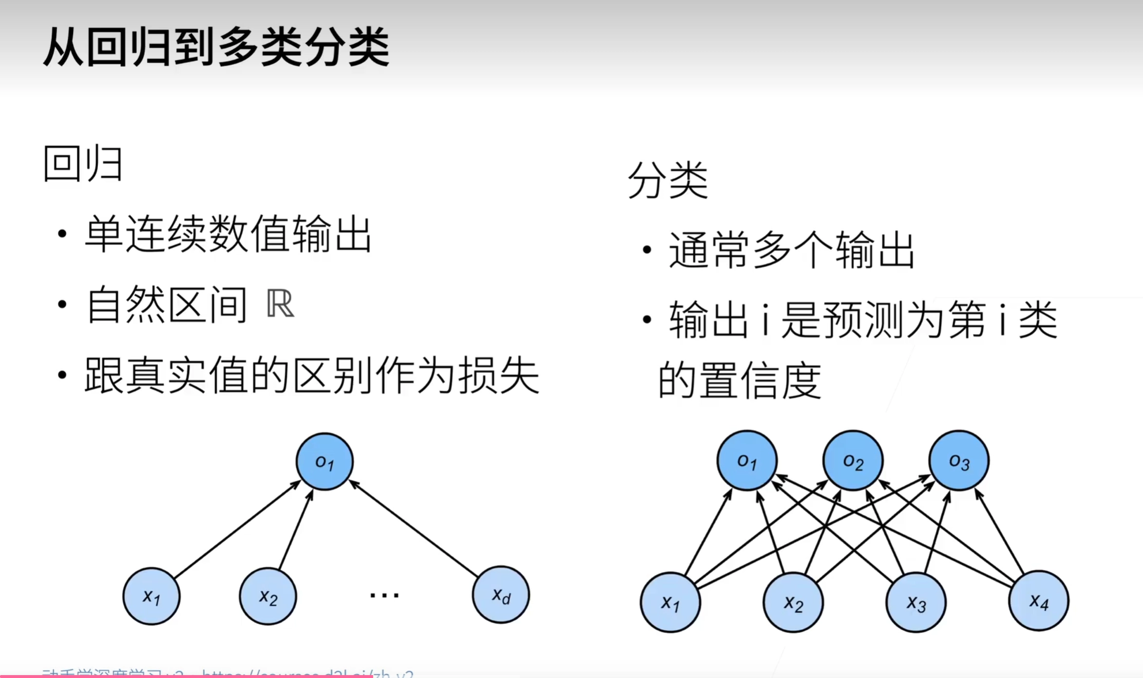
# Softmax回归是分类问题的一种常用方法，它可以将输入的特征映射到一个固定范围的输出上，使得输出的范围在0到1之间，且所有输出的总和为1。
# 如mnist和ImageNet数据集

[

](https://img2024.cnblogs.com/blog/3517150/202505/3517150-20250519230111675-1042372178.png)

In [ ]:


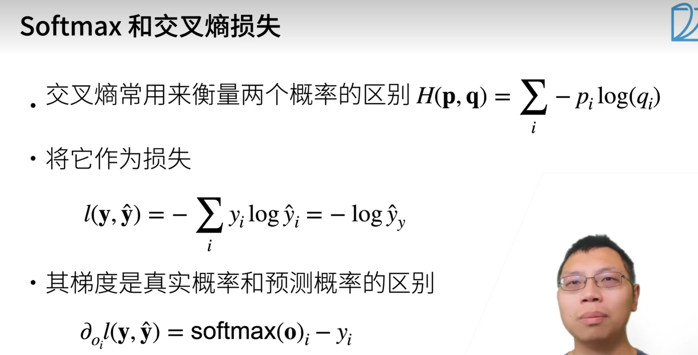
# 就是概率，谁的概率大，谁就是那个物体
# 通过交叉熵损失函数来衡量模型的预测值与真实值之间的差距，并通过反向传播算法来更新模型参数，使得损失函数最小化。

[

](https://img2024.cnblogs.com/blog/3517150/202505/3517150-20250519230111633-1158743210.png)

损失函数¶#

L2 Loss: 0.5 * (y_hat - y)^2

L1 Loss: |y_hat - y|

Huber Loss: L2 Loss if |y_hat - y| <= delta else delta * (|y_hat - y| - 0.5 * delta)

图片分类数据集¶

In [52]:


# 读取Fashion-MNIST数据集
# 通过ToTensor实例将图像数据从PIL类型变换成32位浮点数格式，
# 并除以255使得所有像素的数值均在0～1之间
trans = transforms.ToTensor()
mnist_train = torchvision.datasets.FashionMNIST(
    root="../data", train=True, transform=trans, download=True)
mnist_test = torchvision.datasets.FashionMNIST(
    root="../data", train=False, transform=trans, download=True)
len(mnist_train), len(mnist_test)


100%|██████████| 26.4M/26.4M [00:09<00:00, 2.77MB/s]
100%|██████████| 29.5k/29.5k [00:00<00:00, 114kB/s]
100%|██████████| 4.42M/4.42M [00:02<00:00, 2.10MB/s]
100%|██████████| 5.15k/5.15k [00:00<00:00, 8.62MB/s]

Out[52]:


(60000, 10000)

In [54]:


# 读取第一个图像
mnist_train[0][0].shape  # 1*28*28

Out[54]:


torch.Size([1, 28, 28])

In [55]:


def get_fashion_mnist_labels(labels):  #@save
    """返回Fashion-MNIST数据集的文本标签"""
    text_labels = ['t-shirt', 'trouser', 'pullover', 'dress', 'coat',
                   'sandal', 'shirt', 'sneaker', 'bag', 'ankle boot']
    return [text_labels[int(i)] for i in labels]
def show_images(imgs, num_rows, num_cols, titles=None, scale=1.5):  #@save
    """绘制图像列表"""
    figsize = (num_cols * scale, num_rows * scale)
    _, axes = d2l.plt.subplots(num_rows, num_cols, figsize=figsize)
    axes = axes.flatten()
    for i, (ax, img) in enumerate(zip(axes, imgs)):
        if torch.is_tensor(img):
            # 图片张量
            ax.imshow(img.numpy())
        else:
            # PIL图片
            ax.imshow(img)
        ax.axes.get_xaxis().set_visible(False)
        ax.axes.get_yaxis().set_visible(False)
        if titles:
            ax.set_title(titles[i])
    return axes

In [61]:


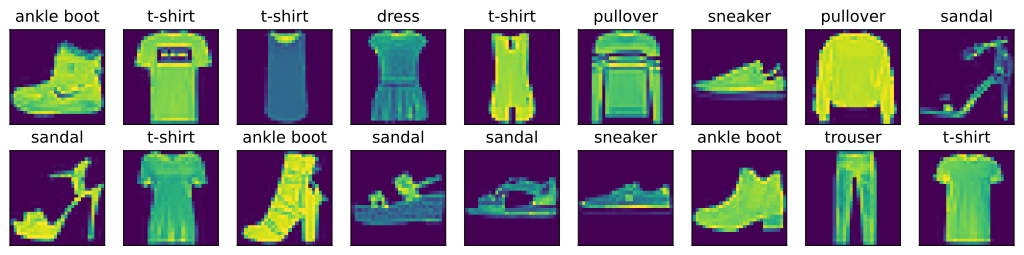
# 加载数据集
X , y=next(iter(data.DataLoader(mnist_train, batch_size=18)))
show_images(X.reshape(18, 28, 28), 2, 9, titles=get_fashion_mnist_labels(y))

Out[61]:


array([<Axes: title={'center': 'ankle boot'}>,
       <Axes: title={'center': 't-shirt'}>,
       <Axes: title={'center': 't-shirt'}>,
       <Axes: title={'center': 'dress'}>,
       <Axes: title={'center': 't-shirt'}>,
       <Axes: title={'center': 'pullover'}>,
       <Axes: title={'center': 'sneaker'}>,
       <Axes: title={'center': 'pullover'}>,
       <Axes: title={'center': 'sandal'}>,
       <Axes: title={'center': 'sandal'}>,
       <Axes: title={'center': 't-shirt'}>,
       <Axes: title={'center': 'ankle boot'}>,
       <Axes: title={'center': 'sandal'}>,
       <Axes: title={'center': 'sandal'}>,
       <Axes: title={'center': 'sneaker'}>,
       <Axes: title={'center': 'ankle boot'}>,
       <Axes: title={'center': 'trouser'}>,
       <Axes: title={'center': 't-shirt'}>], dtype=object)

[

](https://img2024.cnblogs.com/blog/3517150/202505/3517150-20250519230111204-1928288738.svg)

In [62]:


batch_size = 256

def get_dataloader_workers():  #@save
    """使用4个进程来读取数据"""
    return 4

train_iter = data.DataLoader(mnist_train, batch_size, shuffle=True,
                             num_workers=get_dataloader_workers())
timer = d2l.Timer()
for X, y in train_iter:
    continue
f'{timer.stop():.2f} sec'

Out[62]:


'4.81 sec'

整合所有组件¶#

现在我们定义load_data_fashion_mnist函数，用于获取和读取Fashion-MNIST数据集。这个函数返回训练集和验证集的数据迭代器。此外，这个函数还接受一个可选参数resize，用来将图像大小调整为另一种形状。

In [ ]:


def load_data_fashion_mnist(batch_size, resize=None):  #@save
    """下载Fashion-MNIST数据集，然后将其加载到内存中"""
    trans = [transforms.ToTensor()]
    if resize:
        trans.insert(0, transforms.Resize(resize))
    trans = transforms.Compose(trans)
    mnist_train = torchvision.datasets.FashionMNIST(
        root="../data", train=True, transform=trans, download=True)
    mnist_test = torchvision.datasets.FashionMNIST(
        root="../data", train=False, transform=trans, download=True)
    return (data.DataLoader(mnist_train, batch_size, shuffle=True,
                            num_workers=get_dataloader_workers()),
            data.DataLoader(mnist_test, batch_size, shuffle=False,
                            num_workers=get_dataloader_workers()))

In [65]:


train_iter, test_iter = load_data_fashion_mnist(32, resize=64)
for X, y in train_iter:
    print(X.shape, X.dtype, y.shape, y.dtype)
    break


torch.Size([32, 1, 64, 64]) torch.float32 torch.Size([32]) torch.int64

In [ ]:


# Softmax从零开始实现
batch_size = 256
train_iter, test_iter = load_data_fashion_mnist(batch_size)
num_inputs = 784 # 28*28,展平每个图像的像素为一个784维向量
num_outputs = 10 # 10个类
W = torch.normal(0, 0.01, size=(num_inputs, num_outputs), requires_grad=True)
b = torch.zeros(num_outputs, requires_grad=True)
X = np.array([[1.0, 2.0, 3.0], [4.0, 5.0, 6.0]])
X.sum(0, keepdims=True), X.sum(1, keepdims=True) # 按列求和，按行求和

Out[ ]:


(array([[5., 7., 9.]]),
 array([[ 6.],
        [15.]]))

实现softmax由三个步骤组成：

对每个项求幂（使用exp）；

对每一行求和（小批量中每个样本是一行），得到每个样本的规范化常数；

将每一行除以其规范化常数，确保结果的和为1。

In [67]:


def softmax(X):
    X_exp = torch.exp(X)
    partition = X_exp.sum(1, keepdim=True)
    return X_exp / partition  # 这里应用了广播机制

In [68]:


# 实现softmax回归模型
def net(X):
    # 展平每个图像的像素为一个784维向量
    return softmax(torch.matmul(X.view((-1, num_inputs)), W) + b)

In [70]:


# 使用torch.normal生成均值为0，标准差为1的正态分布随机数，形状为(2, 5)
X = torch.normal(0, 1, (2, 5))

# 对X应用softmax函数，将其转换为概率分布
X_prob = softmax(X)

# 输出X_prob和每一行的概率之和，验证softmax后每一行的概率和是否为1
X_prob, X_prob.sum(1)

Out[70]:


(tensor([[0.1315, 0.1987, 0.1105, 0.1217, 0.4376],
         [0.2637, 0.1140, 0.0931, 0.0490, 0.4803]]),
 tensor([1.0000, 1.0000]))

In [71]:


# 定义标签张量y，包含两个样本的类别索引，分别为0和2
y = torch.tensor([0, 2])

# 定义预测概率张量y_hat，包含两个样本在三个类别上的预测概率
y_hat = torch.tensor([[0.1, 0.3, 0.6], [0.3, 0.2, 0.5]])

# 使用y_hat[[0, 1], y]来选择每个样本在其真实类别上的预测概率
# 具体来说，选择第一个样本在类别0上的预测概率（0.1）和第二个样本在类别2上的预测概率（0.5）
y_hat[[0, 1], y]

Out[71]:


tensor([0.1000, 0.5000])

In [ ]:


# 定义交叉熵损失函数
def cross_entropy(y_hat, y):
    return - torch.log(y_hat[range(len(y_hat)), y])

cross_entropy(y_hat, y)

Out[ ]:


tensor([2.3026, 0.6931])

In [73]:


def accuracy(y_hat, y):  #@save
    """计算预测正确的数量"""
    if len(y_hat.shape) > 1 and y_hat.shape[1] > 1:
        y_hat = y_hat.argmax(axis=1)
    cmp = y_hat.type(y.dtype) == y
    return float(cmp.type(y.dtype).sum())

In [74]:


accuracy(y_hat, y) / len(y)

Out[74]:

0.5

In [76]:


def evaluate_accuracy(net, data_iter):  #@save
    """计算在指定数据集上模型的精度"""
    if isinstance(net, torch.nn.Module):
        net.eval()  # 将模型设置为评估模式
    metric = Accumulator(2)  # 正确预测数、预测总数
    with torch.no_grad():
        for X, y in data_iter:
            metric.add(accuracy(net(X), y), y.numel())
    return metric[0] / metric[1]

In [77]:


class Accumulator:  #@save
    """在n个变量上累加"""
    def __init__(self, n):
        self.data = [0.0] * n

    def add(self, *args):
        self.data = [a + float(b) for a, b in zip(self.data, args)]

    def reset(self):
        self.data = [0.0] * len(self.data)

    def __getitem__(self, idx):
        return self.data[idx]

In [79]:


evaluate_accuracy(net, test_iter)

Out[79]:


0.0122

In [81]:


def train_epoch_ch3(net, train_iter, loss, updater):  #@save
    """训练模型一个迭代周期（定义见第3章）"""
    # 将模型设置为训练模式
    if isinstance(net, torch.nn.Module):
        net.train()
    # 训练损失总和、训练准确度总和、样本数
    metric = Accumulator(3)
    for X, y in train_iter:
        # 计算梯度并更新参数
        y_hat = net(X)
        l = loss(y_hat, y)
        if isinstance(updater, torch.optim.Optimizer):
            # 使用PyTorch内置的优化器和损失函数
            updater.zero_grad()
            l.mean().backward()
            updater.step()
        else:
            # 使用定制的优化器和损失函数
            l.sum().backward()
            updater(X.shape[0])
        metric.add(float(l.sum()), accuracy(y_hat, y), y.numel())
    # 返回训练损失和训练精度
    return metric[0] / metric[2], metric[1] / metric[2]

In [87]:


from IPython import display

In [88]:


class Animator:  #@save
    """在动画中绘制数据"""
    def __init__(self, xlabel=None, ylabel=None, legend=None, xlim=None,
                 ylim=None, xscale='linear', yscale='linear',
                 fmts=('-', 'm--', 'g-.', 'r:'), nrows=1, ncols=1,
                 figsize=(3.5, 2.5)):
        # 增量地绘制多条线
        if legend is None:
            legend = []
        d2l.use_svg_display()
        self.fig, self.axes = d2l.plt.subplots(nrows, ncols, figsize=figsize)
        if nrows * ncols == 1:
            self.axes = [self.axes, ]
        # 使用lambda函数捕获参数
        self.config_axes = lambda: d2l.set_axes(
            self.axes[0], xlabel, ylabel, xlim, ylim, xscale, yscale, legend)
        self.X, self.Y, self.fmts = None, None, fmts

    def add(self, x, y):
        # 向图表中添加多个数据点
        if not hasattr(y, "__len__"):
            y = [y]
        n = len(y)
        if not hasattr(x, "__len__"):
            x = [x] * n
        if not self.X:
            self.X = [[] for _ in range(n)]
        if not self.Y:
            self.Y = [[] for _ in range(n)]
        for i, (a, b) in enumerate(zip(x, y)):
            if a is not None and b is not None:
                self.X[i].append(a)
                self.Y[i].append(b)
        self.axes[0].cla()
        for x, y, fmt in zip(self.X, self.Y, self.fmts):
            self.axes[0].plot(x, y, fmt)
        self.config_axes()
        display.display(self.fig)
        display.clear_output(wait=True)
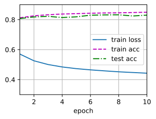
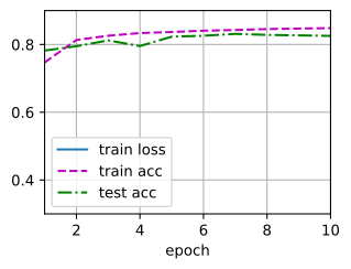
def train_ch3(net, train_iter, test_iter, loss, num_epochs, updater):  #@save
    """训练模型（定义见第3章）"""
    animator = Animator(xlabel='epoch', xlim=[1, num_epochs], ylim=[0.3, 0.9],
                        legend=['train loss', 'train acc', 'test acc'])
    for epoch in range(num_epochs):
        train_metrics = train_epoch_ch3(net, train_iter, loss, updater)
        test_acc = evaluate_accuracy(net, test_iter)
        animator.add(epoch + 1, train_metrics + (test_acc,))
    train_loss, train_acc = train_metrics
    assert train_loss < 0.5, train_loss
    assert train_acc <= 1 and train_acc > 0.7, train_acc
    assert test_acc <= 1 and test_acc > 0.7, test_acc

In [89]:


lr = 0.1

def updater(batch_size):
    return d2l.sgd([W, b], lr, batch_size)

In [90]:


num_epochs = 10
train_ch3(net, train_iter, test_iter, cross_entropy, num_epochs, updater)

[

](https://img2024.cnblogs.com/blog/3517150/202505/3517150-20250519230111153-725344193.svg)

In [92]:


def predict_ch3(net, test_iter, n=20):  #@save
    """预测标签（定义见第3章）"""
    for X, y in test_iter:
        break
    trues = d2l.get_fashion_mnist_labels(y)
    preds = d2l.get_fashion_mnist_labels(net(X).argmax(axis=1))
    titles = [true +'\n' + pred for true, pred in zip(trues, preds)]
    d2l.show_images(
        X[0:n].reshape((n, 28, 28)), 1, n, titles=titles[0:n])

predict_ch3(net, test_iter)

[

](https://img2024.cnblogs.com/blog/3517150/202505/3517150-20250519230111198-1164068632.svg)

In [ ]:


# softmax回归的简洁实现
batch_size = 256
train_iter, test_iter = d2l.load_data_fashion_mnist(batch_size)

In [94]:


import torch
import torch.nn as nn
import torch.optim as optim

# 定义一个顺序容器，其中包含两个层：
# 1. 展平层（Flatten）：将输入的多维数据展平成一维向量。
# 2. 线性层（Linear）：一个全连接层，输入特征为784维（例如28x28的图像展平为784维），输出特征为10维（例如10个类别）。
net = nn.Sequential(nn.Flatten(), nn.Linear(784, 10))  # 定义展平层

# 定义一个初始化权重的函数
def init_weights(m):
    # 检查当前模块是否为线性层
    if type(m) == nn.Linear:
        # 使用正态分布初始化线性层的权重，均值为0，标准差为0.01
        nn.init.normal_(m.weight, mean=0, std=0.01)
        # 将线性层的偏置初始化为0
        nn.init.zeros_(m.bias)

# 应用初始化权重的函数到网络的每一层
net.apply(init_weights)  # 初始化权重

# 定义损失函数为交叉熵损失函数，常用于多分类问题
loss = nn.CrossEntropyLoss()  # 交叉熵损失函数

# 定义优化器为随机梯度下降（SGD），并设置学习率为0.1
optimizer = torch.optim.SGD(net.parameters(), lr=0.1)  # 随机梯度下降优化器

# 设置训练的轮数为10
num_epochs = 10  # 设置训练轮数
train_ch3(net, train_iter, test_iter, loss, num_epochs, optimizer)  # 训练模型

[

](https://img2024.cnblogs.com/blog/3517150/202505/3517150-20250519230111111-222902215.svg)

In [ ]:

损失函数¶#

图片分类数据集¶

整合所有组件¶#

相关文章